Automatic Design of SARS-CoV-2 Mpro Inhibitors via Machine Learning & Molecular Docking
Published:
Introduction
One of my current interest is in developing machine learning (ML) methods for optimizing chemical processes. Recently, in collaboration with the folks over at Princeton and Bristol Myers Squibb, I finished writing a python package called Experimental Design via Bayesian Optimization (EDBO) for reaction optimization which enables the application of Bayesian optimization, an uncertainty guided response surface method, to chemical reactions in the laboratory. While the software was developed with this specific application in mind, it is a general implementation and I was curious what other fun tasks it might interface with.
As a synthetic chemist I have heard quite a bit about docking simulations and the role they play in the drug discovery process. In this context, docking refers to molecular modeling methods which enable the prediction of binding affinity between a drug-like molecule and a biological target such as a protein. In turn, the predicted binding behavior and conformation can enable chemists and biologists to identify promising structures for experimental evaluation and potential small molecule therapeutics. With this general understanding, the objective of this post is to get a little hands on experience. Specifically, we will take a quick dive into the process of molecular docking using open-source tools. And to make things even more fun we will also put together a fully automated artificial intelligence (AI) based ligand discovery pipeline using EDBO, run it on my laptop, and see what it discovers!
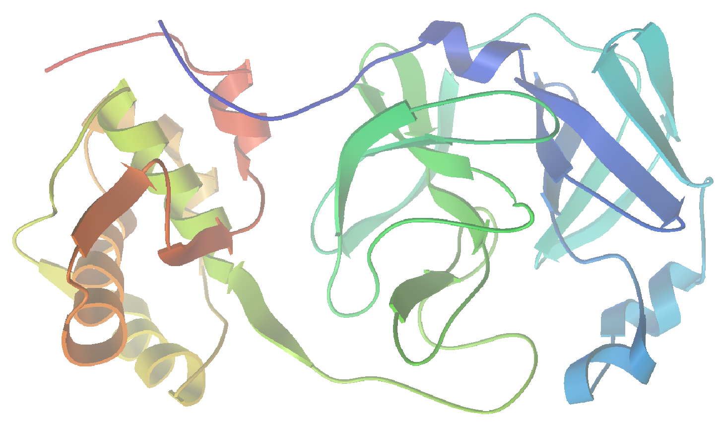
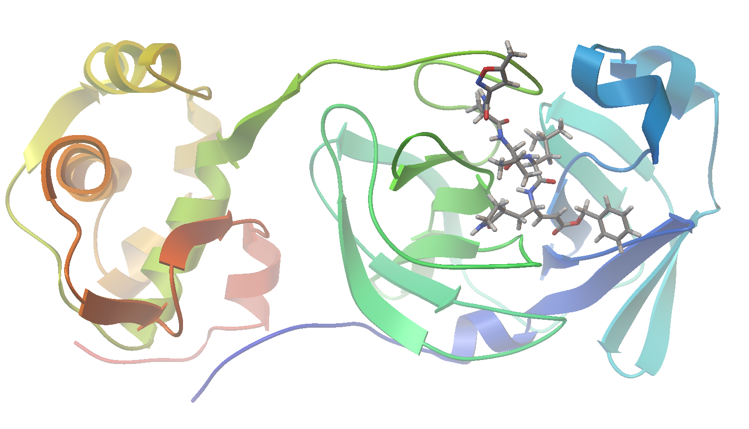
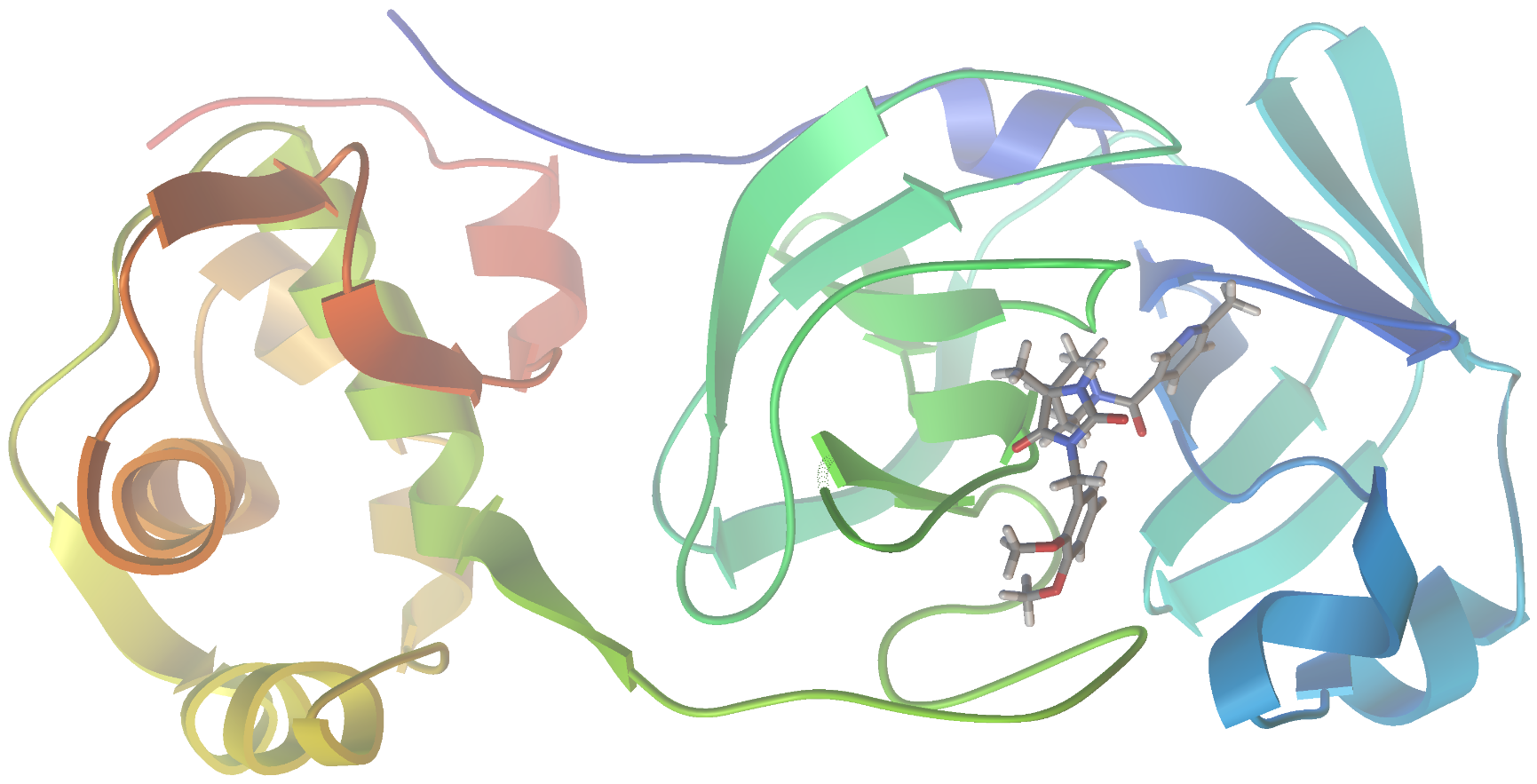
As I am writing this post, we are in the midst of the covid-19 pandemic. Accordingly, I could see no better target for this project than SARS-CoV-2, the virus responsible for our current situation. In a recent report (Jin, et al. “Structure of Mpro from SARS-CoV-2 and discovery of its inhibitors” Nature, 2020, 582,289), researchers disclosed the identification of several SARS-CoV-2 inhibitors of Mpro, a protease enzyme critical to the replication cycle of SARS-CoV-2. The polyproteins responsible for viral replication and transcription must undergo proteolytic processing (digestion) by Mpro. Thus, Mpro is an ideal target for antiviral drugs. A ribbon structure of Mpro is shown below.
In order to pull this off we need to code a few key components including: (1) a molecular structure generator - converts from a string representation to 3D coordinates, carries out geometry optimization, and generates conformers, (2) a molecular docking simulator - submits generated structures and return a binding score, and (3) an automated AI optimizer - optimizes molecular structure to maximize binding score. In turn, the AI method requires: (A) a search space - chemical space to optimize over, (B) an encoding - numerical representation of molecular structures, and (C) an optimizer - selects the next experiments to run according to some utility function. For the search space and encoding I thought it would be interesting to use a variational autoencoder (vide infra), trained on the structures for drug-like molecules, to generate a numerical embedding for optimization.
Automating 3D structure generation
Generating representative 3D molecular structures from SMILES strings is critical for this application. This is because we are going to use a variational autoencoder trained on SMILES strings. In addition, I wanted to code this application in python and avoid quantum mechanical (e.g., DFT) geometry optimization. Therefore, let’s use Open-Babels python API to generate 3D structures from smiles strings via: (1) creating the initial structure using rules and fragment templates, (2) steepest descent geometry optimization with the MMFF94 forcefield, (3) a weighted rotor conformational search, and (4) and a final conjugate gradient geometry optimization on the lowest energy conformer. Then additional geometries can be generated using open-babels built in genetic algorithm for diverse conformer generation. Let’s wrap all of the methods we will need up into one handy python class. You can see the details for each method in the accompanying doc strings.
from openbabel import pybel
import re

# Molecule class handles structure generation, conformer searching, and input generation

class molecule:
    """
    Class for handling structure generation and conformer searching.
    The methods defined here will allow us to generate 3D coordinates
    to feed into docking simulations.
    """

    def __init__(self, SMILES, NAME, correct_for_ph=True, ph=7.4):

        # Save SMILES and NAME
        self.smi = SMILES
        self.name = NAME
        self.correct_ph = correct_for_ph
        self.ph = ph

        # Open-Babel
        self.conv = pybel.ob.OBConversion()
        self.obmol = self.smiles_to_obmol()
        self.obmol.AddHydrogens()
        if correct_for_ph:
            self.obmol.CorrectForPH(ph)
        self.obmol.SetTitle(self.name)

    def smiles_to_obmol(self, input_format='smi'):
        """
        Convert a SMILES string to an obmol object.
        """

        mol = pybel.ob.OBMol()
        self.conv.SetInFormat(input_format)
        self.conv.ReadString(mol, self.smi)

        return mol

    def to_string(self, output_format='mol2'):
        """
        Using the current obmol object generate a formatted
        string.
        """

        self.conv.SetOutFormat(output_format)
        out = self.conv.WriteString(self.obmol).strip()

        return out

    def to_file(self, path, confs=False, output_format='mol2'):
        """
        Write formatted structure data for optimized geometries.
        """

        if confs:
            # Open output file
            file = pybel.Outputfile(output_format,
                                    path + '.' + output_format,
                                    overwrite=True)

            # Write conformers
            for c in range(self.n_confs):
                # Conformer name
                self.obmol.SetConformer(c)
                self.obmol.SetTitle(self.name + str(c))
                file.write(pybel.Molecule(self.obmol))

            # Close file
            file.close()
        else:
            self.conv.SetOutFormat(output_format)
            self.conv.WriteFile(self.obmol, path + '.' + output_format)

        # Reset name
        self.obmol.SetTitle(self.name)

    def _geom(self):
        """
        Generate a starting geometry.
        """

        # Initial generation
        gen3D = pybel.ob.OBOp.FindType("gen3D")
        gen3D.Do(self.obmol, 'best')

        # Sometimes this fails so we need to check for proper 3D coordinates
        txt = self.to_string(output_format='xyz')
        coord = re.findall('[\d]+', txt)
        if len(set(coord)) < 10:
            pybel.Molecule(self.obmol).make3D(forcefield='mmff94',
                                              steps=250)

    def conf_gen(self, n_confs=30):
        """
        Run a conformer generation generating up to n_confs
        conformers.
        """

        self._geom()

        confSearch = pybel.ob.OBConformerSearch()
        confSearch.Setup(self.obmol, n_confs)
        confSearch.Search()
        confSearch.GetConformers(self.obmol)

        self.n_confs = self.obmol.NumConformers()
We can run a quick test of the class and its methods using a known binder of Mpro (called N3 in the recent paper). Here is an example block of code to instantiate a molecule, generate conformers, and write them to a MOL2 file.
m = molecule('O=C(N[C@@H](C)C(N[C@@H](C(C)C)C(N[C@@H](CC(C)C)C(N[C@H](/C=C/C(OCC1=CC=CC=C1)=O)C[C@@H]2CCNC2=O)=O)=O)=O)C3=NOC(C)=C3', 'N3')
m.conf_gen(n_confs=3)
m.to_file(m.name, confs=True)
Molecular docking simulations
Next, we require a docking simulator and python interface which takes conformations of a given molecule as an input and return a predicted binding affinity. For the docking simulations we will use the freely available software AutoDock Vina. Autodock Vina computes a binding score via a scoring function that approximates the chemical potential of the system (Trott et al. “AutoDock Vina: improving the speed and accuracy of docking with a new scoring function, efficient optimization and multithreading”, J. Comput. Chem., 2010, 31, 455). However, recently it has been demonstrated that including an additional machine learning (ML) based scoring function, trained on active and inactive molecules docked to a large set of targets, as a post-processing step can give substantial improvements in virtual screening performance in terms of hit rate (Wójcikowski et al. “Performance of machine-learning scoring functions in structure-based virtual screening”, Scientific Reports, 2017, 7, 46710). Here we will use RF-Score (a random forest scoring function) which takes as input the AutoDock output and returns an adjusted score. Notably, using AutoDock Vina for molecular docking and Open Drug Discovery Toolkit as a python interface this whole pipeline is actually pretty straightforward to implement.
Let’s write a python class which: (1) parses input for an arbitrary protein, bound ligand, and candidate ligands, (2) interfaces with AutoDock Vina to run docking simulations, (3) computes the RF-Score from the output, and (4) parses the results (which come in the form of MOL2 files) to return scores and docked structures. You can see the function of each method in the accompanying doc strings.
from oddt.virtualscreening import virtualscreening as vs
import os
import shutil
import re
import pandas as pd

# Docking class handles automatic docking and output parsing

class dock:
    """
    Class for handling automated docking simulations, file manipulations,
    and result parsing.
    """

    def __init__(self, protein, protein_ligand, ligands, n_cpu=-1):

        # Input file paths
        self.protein = protein
        self.protein_ligand = protein_ligand
        self.ligands = ligands
        self.executable = 'PATH_TO_VINA.EXE'

        # Virtual screening pipeline
        self.pipeline = vs(n_cpu=n_cpu)

        # Load ligands from a mol2 file
        self.pipeline.load_ligands('mol2', self.ligands)

        # Dock entire library to receptor, autocenter docking box on ligand
        self.pipeline.dock('autodock_vina',
                           self.protein,
                           self.protein_ligand,
                           executable=self.executable)

        # Post-processing using a scoring function
        self.pipeline.score(function='rfscore',
                            protein=self.protein,
                            version=1)

    def run(self, output_file, overwrite=False):
        """
        Run docking simulation for a given protein and ligand.
        """

        # Unique output file name
        output_file += '.mol2'

        # If you don't want to overwrite previous output
        if overwrite == False:
            counter = 1
            while os.path.isfile(output_file):
                parts = output_file.split('.')
                parts[0] += str(counter)
                counter += 1
                output_file = parts[0] + '.' + parts[1]

        # Run docking simulation and write output
        self.pipeline.write('mol2',
                            output_file,
                            # overwrite=True,
                            opt={'c':None})

        # Get results text
        f = open(output_file, 'r')
        self.results_text = f.read()
        f.close()
        self.parse_results()
        self.clean_dir()

    def parse_results(self):
        """
        Parse docking output to get Vina docking scores and
        scoring function results.
        """

        # Break file up into each conformer
        mols = self.results_text.split('\n\n##########')

        # Extract results for each
        results = []
        for mol in mols:

            # Get scores
            output = re.findall(r'\t(.+):\t([0-9]+[.]?[0-9]+)', mol)
            names = re.findall(r'MOLECULE\n(.+)\n', mol)

            # Tabulate results
            columns = ['Conformer']
            tabulated = [names[0]]
            for entry in output:
                columns.append(entry[0])
                tabulated.append(entry[1])

            results.append(pd.DataFrame([tabulated], columns=columns))

        # Generate a results DataFrame
        self.results = pd.DataFrame(columns=results[0].columns.values)
        for entry in results:
            self.results = pd.concat([self.results, entry])

        # Make sure RF Score is the last column
        last = 0
        while 'score' not in self.results.columns.values[last]:
            last += 1

        self.results = self.results.iloc[:,:last + 1]

    def write_conformer(self, conformer_number):
        """
        Write a docked conformer to a .mol2 file. Use this to
        visualize docked ligand conformations in PMV.
        """

        f = open('conf.mol2', 'w')
        f.write(self.results_text.split('\n\n##########')[conformer_number])
        f.close()

    def write_best_conformer(self):
        """
        Parse results for conformer with best score and write
        coordinates to a .mol2 file for evaluation.
        """

        best = self.results.sort_values(self.results.columns.values[-1]).iloc[[-1]].index.values[0]
        self.write_conformer(best)

    def clean_dir(self):
        """
        Garbage collector. In some cases I have seen exceptions b/c
        oddt wasn't able to remove temporary files.
        """

        # Get files in cwd
        files = [x[0].split('\\')for x in os.walk('.')]

        # Try to remove temporary files
        try:
            for file in files:
                if len(file) == 2:
                    if 'autodock_vina' in file[1]:
                        shutil.rmtree(file[1])
        except Exception as e:
            print(e)
            if 'cannot access' in str(e):
                print('Could not remove temporary files...')
                pass
Now, for our particular problem we need structural data for Mpro with a bound ligand (N3). We can get this from the recent publication’s supplemental information (vide supra). With the raw data in hand, we then need to prepare the individual protein and bound ligand structure data (PDBQT files) for modeling using Python Molecular Viewer (PMV) (e.g., by removing water molecules, adding hydrogens, and generating a grid). I did this by following the tutorial on the AutoDock Vina website. Then to test our docking class we will run simulations using the N3 structures generated with the molecule class above.
protein = 'proteins/6lu7_protein.pdbqt'          # Protein structure
protein_ligand = 'proteins/6lu7_ligand.pdbqt'    # Bound ligand structure
ligands = m.name + '.mol2'                       # Structures generated with molecule class

d = dock(protein, protein_ligand, ligands)
d.run(m.name + '_docking')
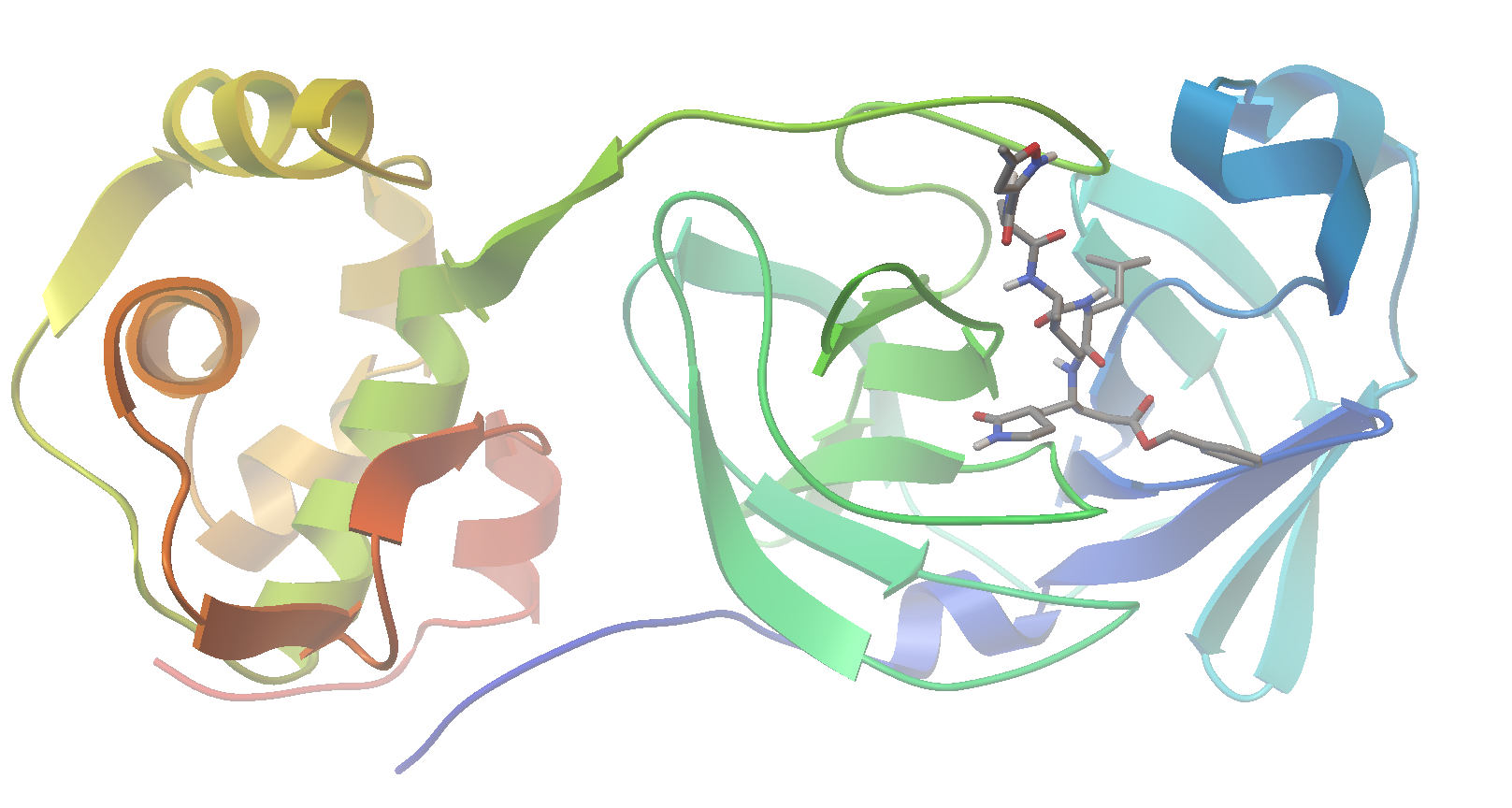
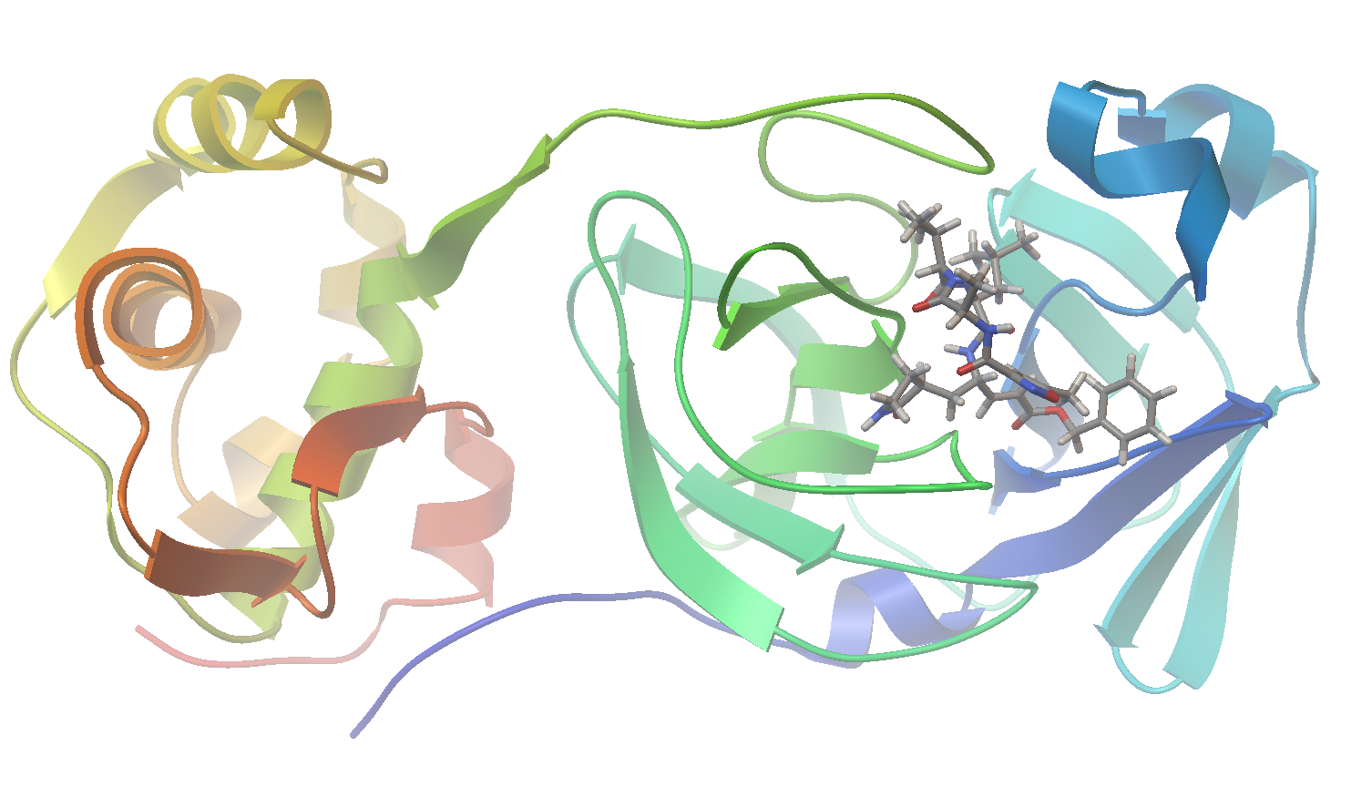
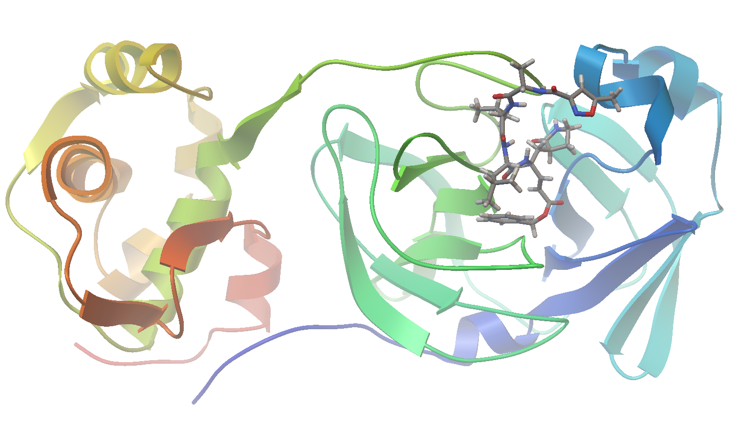
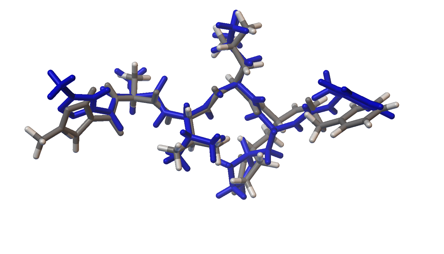
Now let’s visualize the results for the best predicted binding mode of N3 using PMV. You can see that the predicted structure fits nicely in the binding pocket and that the conformation with the best predicted binding affinity has good agreement with the experimental structure.
Crystal Structure:
Sample of Predicted Binding Modes:
Structure Overlay:
Variational autoencoder
The next piece of the puzzle is the variational autoencoder which is used to convert SMILES representations of molecules to and from a continuous numerical encoding. Importantly, this model will allow us to run an optimization in the continuous representation while decoding to discrete chemical structures. We will use an autoencoder trained using drug-like molecules from a recent paper for this demonstration (Gómez-Bombarelli et al. “Automatic Chemical Design Using a Data-Driven Continuous Representation of Molecules”, ACS Cent. Sci., 2018, 4, 268). Here is some example code from the authors repository for encoding and decoding SMILES strings:
from os import environ
environ['KERAS_BACKEND'] = 'tensorflow'
from chemvae.vae_utils import VAEUtils
from chemvae import mol_utils as mu
import numpy as np
import pandas as pd

# Load model from paper
vae = VAEUtils(directory='chemical_vae-master/models/zinc_properties')

# Encode a SMILES string
smiles = mu.canon_smiles('CSCC(=O)NNC(=O)c1c(C)oc(C)c1C')
X = vae.smiles_to_hot(smiles, canonize_smiles=True)
z = vae.encode(X)

# Decode a point in the continuous embedding
df = vae.z_to_smiles(z, decode_attempts=100, noise_norm=5.0)

print('Found {:d} unique mols, out of {:d}.'.format(len(set(df['smiles'])),sum(df['count'])))
Bayesian optimization
Bayesian optimization is an iterative response surface-based global optimization algorithm which has demonstrated excellent performance in a number of tasks (Shahriari et al. “Taking the Human Out of the Loop: A Review of Bayesian Optimization”, Proceedings of the IEEE, 2016, 104, 148). In a recent collaboration, we developed a framework for Bayesian optimization that is compatible with encoded chemical data and an open-source python software tool that enables easy integration with a given task (EDBO).
Below is a brief demonstration of an arbitrary 1D objective with a discretized domain. While EDBO is designed to work with human-in-the-loop experimentation you can also use computational objectives (we also demonstrate this feature below). Let’s start by defining the simulation functions.
import numpy as np
import pandas as pd
import matplotlib.pyplot as plt
from gpytorch.priors import GammaPrior
from edbo.bro import BO

# Define a computational objective
def f(x):
    """Noise free objective."""

    return np.sin(10 * x[0]) * x[0] * 100

# Bayesian optimization
X = np.linspace(0,1,1000).reshape(1000, 1)
domain = pd.DataFrame(X, columns=['x'])                        # Search space

bo = BO(domain=domain,                                         # Search space
        target='f(x)',                                         # Name of target (not required but nice)
        acquisition_function='EI',                             # Acquisition function
        init_method='rand',                                    # Initialization method
        lengthscale_prior=[GammaPrior(1.2,1.1), 0.2],          # GP length scale prior and initial value
        noise_prior=None,                                      # No noise prior
        batch_size=2,                                          # Number of experiments to choose in parallel
        fast_comp=True,                                        # Use gpytorch fast computation features
        computational_objective=f)                             # The objective is defined as a function

# Plot model and some posterior predictive samples
def plot_results(export_path):
    """Plot summary of 1D BO simulations"""

    mean = bo.obj.scaler.unstandardize(bo.model.predict(bo.obj.domain))                             # GP posterior mean
    std = np.sqrt(bo.model.variance(bo.obj.domain)) * bo.obj.scaler.std * 2                         # GP posterior standard deviation
    samples = bo.obj.scaler.unstandardize(bo.model.sample_posterior(bo.obj.domain, batch_size=3))   # GP samples
    next_points = bo.obj.get_results(bo.proposed_experiments)                                       # Next points proposed by BO
    results = bo.obj.results_input()                                                                # Results for known data

    plt.figure(1, figsize=(8,8))

    # Model mean and standard deviation
    plt.subplot(211)
    plt.plot(X.flatten(), [f(x) for x in X], color='black')
    plt.plot(X.flatten(), mean, label='GP')
    plt.fill_between(X.flatten(), mean-std, mean+std, alpha=0.4)

    # Known results and next selected point
    plt.scatter(results['x'], results['f(x)'], color='black', label='known')
    plt.scatter(next_points['x'], next_points['f(x)'], color='red', label='next_experiments')
    plt.ylabel('f(x)')

    # Samples
    plt.subplot(212)
    for sample in samples:
        plt.plot(X.flatten(), sample.numpy())
    plt.xlabel('x')
    plt.ylabel('Posterior Samples')

    plt.savefig(export_path + '.svg', format='svg', dpi=1200, bbox_inches='tight')
    plt.show()
Now we can run a single round of Bayesian optimization and visualize the results in terms of the selected points and models fit and samples from the posterior predictive distribution.
# Run a single iteration and plot results
bo.init_sample(append=True, seed=4)
bo.run()
plot_results('bo_demo1')
And to to run a simulation for an arbitrary number of iterations we can use the simulate method.
# Run a simulation and plot results
bo.simulate(iterations=5, seed=4)
plot_results('bo_demo2')
Final Modeling Pipeline
Selecting the initial search space. To start we want to get a general idea of the molecular structures which are predicted to bind tightly to Mpro. To do this I carried out an initial search over drug-like molecules in the Zinc database, encoded using the VAE, using Bayesian optimization. A rigorous application may run the optimization over the entire Zinc database (after filtering by criteria of interest like Lipinski’s rule of five), using a HPC cluster to expedite to calculations. However, I am running this demonstration on a 2 core i3 laptop with 8 GB of RAM so I restrict the initial search space to 10,000 randomly sampled points.
from edbo.utils import Data

molecule_grid_size = 10000

# Sample autoencoder
Z, data, smiles = vae.ls_sampler_w_prop(size=molecule_grid_size, return_smiles=True)

# Define and standardize domain
domain = Data(pd.DataFrame(Z, columns=['z' + str(i) for i in range(len(Z[0]))]))
domain.base_data.insert(0, 'SMILES', smiles)
domain.clean()
domain.standardize(scaler='minmax', target=None)
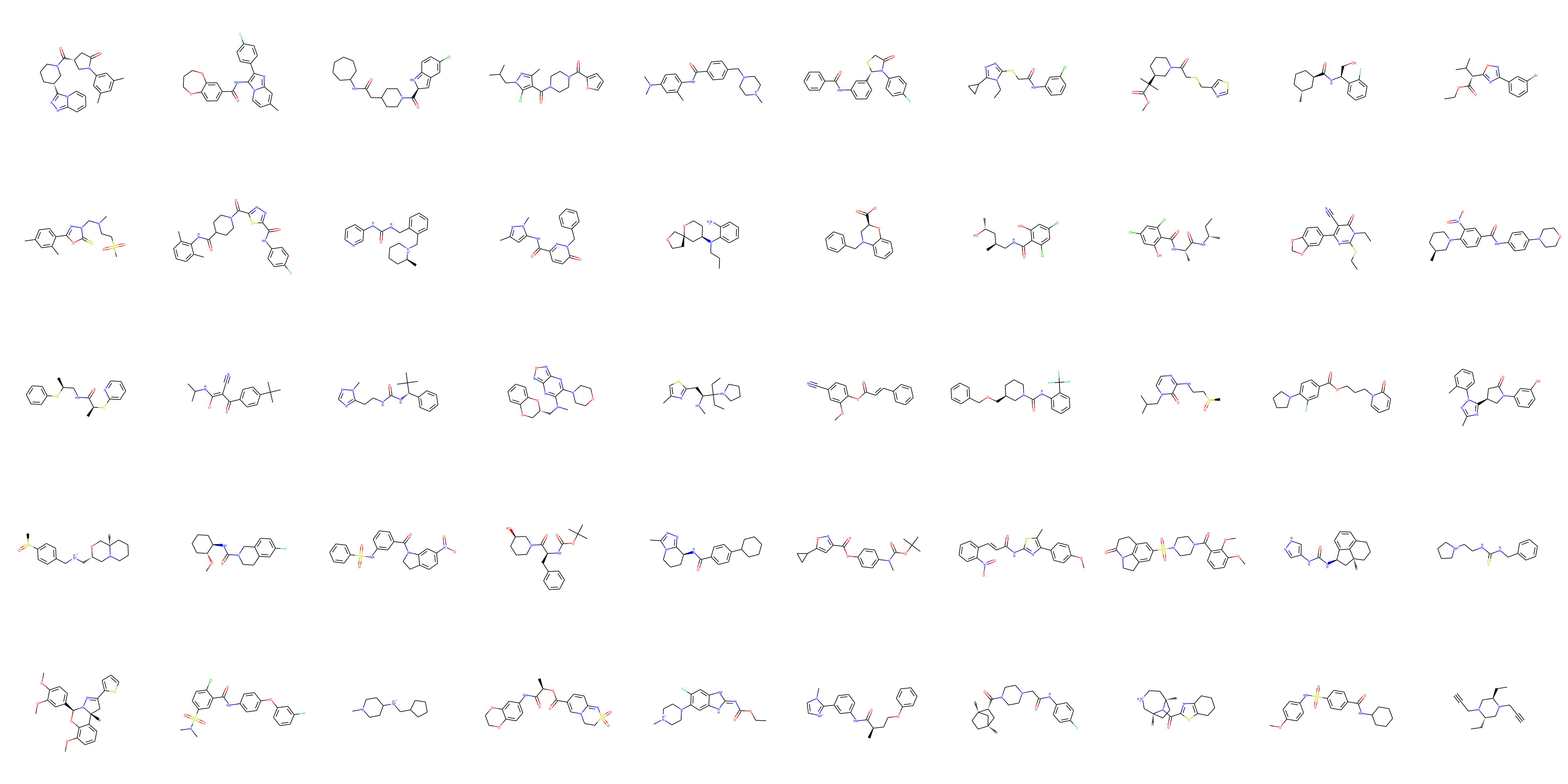
A sample of the selected structures can be seen below:
Optimization. Next we will need to define the computational objective to optimize. To do this we will utilize the molecule class to generate structures, the dock class to run docking simulations, and return the RF-Score for the tightest binding conformer of the molecule.
def best_docking_score(x, n_confs=3):
    """
    Objective function to be used for Bayesian optimization. Returns the predicted binding affinity for the conformer conformer which
    binds best to the Mpro.
    """

    # find correspondence to initial Z matrix
    index = domain.data.where(domain.data == x).dropna().index.values[0]

    # Get SMILES
    smiles = domain.base_data['SMILES'].iloc[index]

    # Print molecule
    cdx = ChemDraw([smiles])
    cdx.show()

    # Get structures
    name = 'step_' + str(index)
    m = molecule(smiles, name)
    m.conf_gen(n_confs=n_confs)
    m.to_file(name, confs=True)

    # Run docking - deal with some exceptions
    try:
        protein = 'proteins/6lu7_protein.pdbqt'           # Protein (delete water, add all H, merge non-polar, grid-->macromol-->choose)
        protein_ligand = 'proteins/6lu7_ligand.pdbqt'     # Protein + bound ligand structure - protein
        ligands = m.name + '.mol2'                        # Candidate ligand structures for binding
        d = dock(protein, protein_ligand, ligands)
        d.run(name + '_docking')
        score = d.results.sort_values(d.results.columns.values[-1]).iloc[-1].values[-1]
    except Exception as e:
        if 'cannot access' in str(e):
            print(e)
            score = best_docking_score(x)
        else:
            score = 4

    return float(score)
Now with this computational objective in hand we can run an initial Bayesian optimization over the randomly sampled search space. Since this is just a demonstration, we will just run the optimizer from a single initial starting point randomly selected from the domain. Keep in mind that in practice it would be better to initialize the optimization with numerous points and to utilize a larger search space.
from edbo.bro import BO

bo = BO(domain=domain.data,
        computational_objective=best_docking_score,
        batch_size=1,
        target='score')

bo.simulate(seed=0, iterations=45)
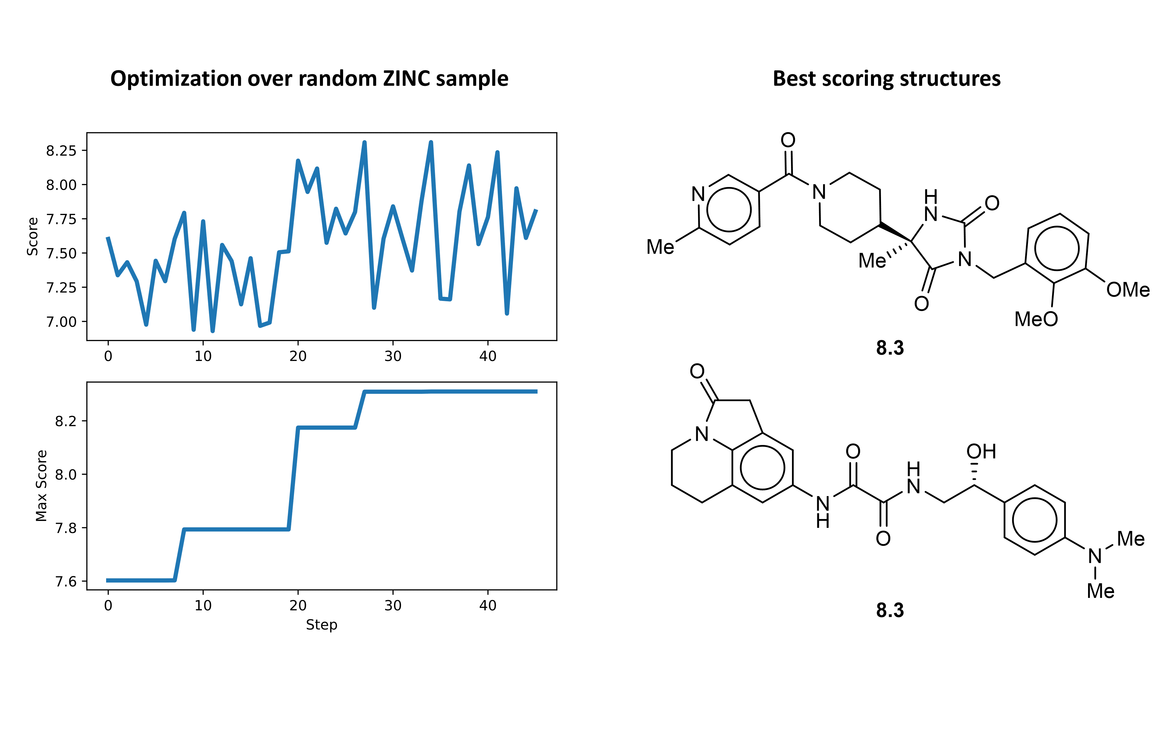
Now we can plot the optimization results in terms of the scores for each molecule and visualize the best scoring ligand. Interestingly, the initially selected molecule actually had a reasonably high docking score. However, over the course of the initial optimization we are still able to see an improvement in predicted binding affinity.
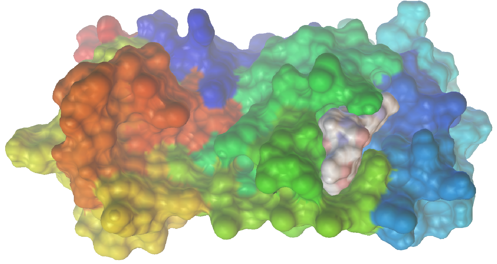
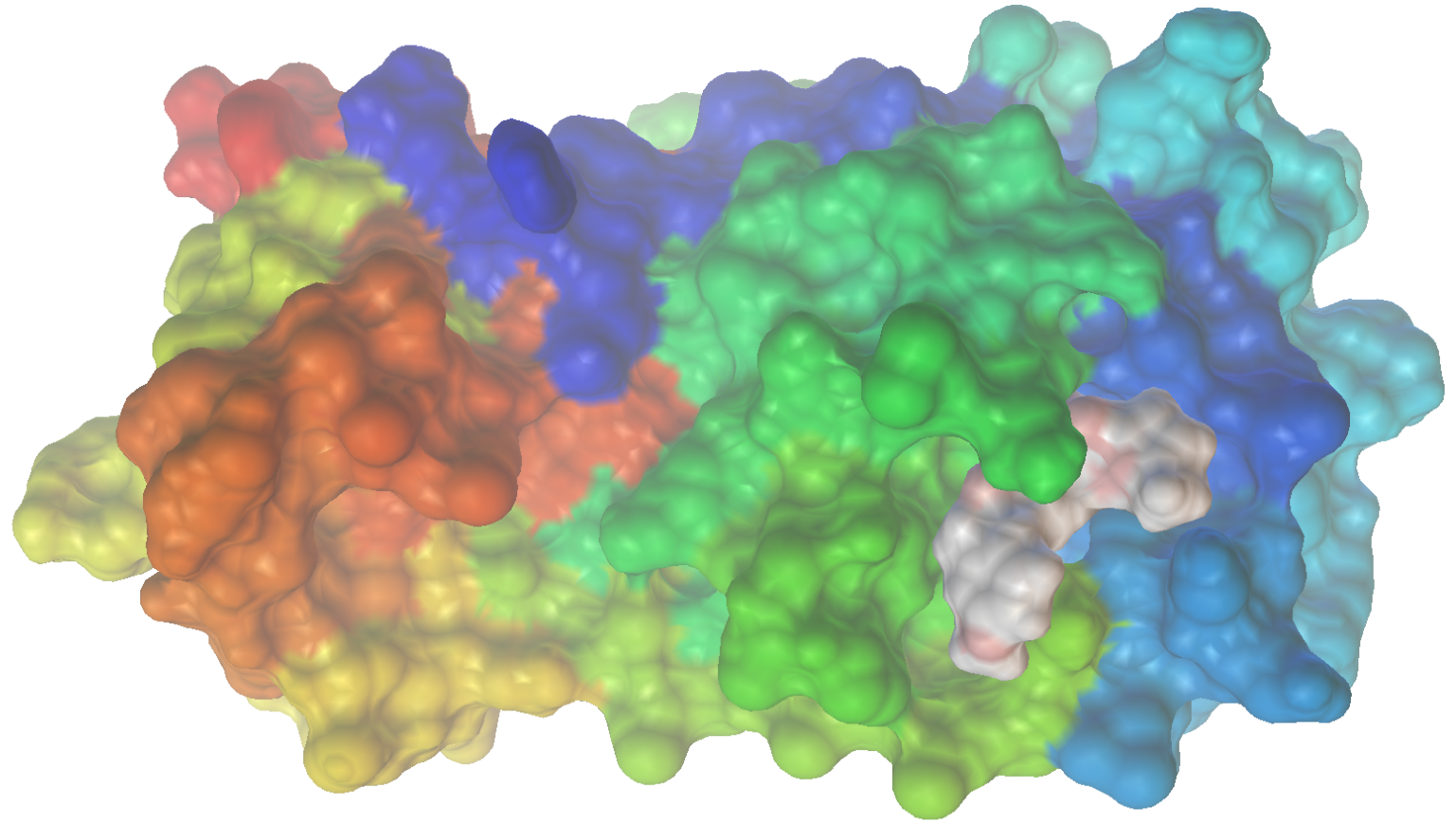
We can dive deeper into the results by visualizing the ligand conformer for the best conformation using PMV. What is very nice to see in the space filling model is that the identified structure actually fits very nicely into the binding site.
Local optimization. As a final step, we can run a more fine grained optimization by using the VAE to generate a new search space centered on one of the interesting structures identified in the initial optimization. Let’s do this by first decoding randomly sampled points in the embedded space about the structure of interest. Then, we can generate additional structures branching out from this region of the space in rounds by carrying out the same procedure over each of the initially decoded points. Finally, the resulting list of structures will define the new search space. The following code will allow us to carry out this local expansion procedure.
def local_search_space(SMILES, noise_norm=10.0, decode_attempts=250, n_points=100):
    """
    Generate a list of similar structures by sampling random points about a given SMILES string
    in the encoded space. Returns the encoded space as a pandas.DataFrame.
    """

    # Encode smiles
    smiles = mu.canon_smiles(SMILES)
    X = vae.smiles_to_hot(smiles, canonize_smiles=True)
    z = vae.encode(X)

    # Randomly sample about point
    # print('Searching molecules randomly sampled from {:.2f} std (z-distance) from the point...'.format(noise_norm))
    df = vae.z_to_smiles(z,
                         decode_attempts=decode_attempts,
                         noise_norm=noise_norm,
                         n_points=n_points,
                         constant_norm=False)
    #print('Found {:d} unique molecules, out of {:d}.'.format(len(set(df['smiles'])),sum(df['count'])))

    return df

def mutate_search_space(SMILES, n_mutations=1, noise_norm=10.0, decode_attempts=250):
    """
    Carries out a series of local searches iteratively and returns a list of SMILES strings.
    """

    smiles_list = [[SMILES]]
    out = [SMILES]

    # Run mutations over identified smiles
    for i in range(n_mutations + 1):
        expansion = []
        for smi in smiles_list[-1]:
            smiles = local_search_space(smi,
                                        noise_norm=noise_norm,
                                        decode_attempts=decode_attempts)['smiles'].drop_duplicates().values
            expansion = expansion + list(smiles)

        expansion = list(set(expansion))
        print('Mutation round ' + str(i) + ':', 'Identified ' + str(len(expansion)) + ' unique structures...')
        smiles_list.append(expansion)
        out = out + list(expansion)

    # Remove initial point
    out = list(set(out) - set([SMILES]))

    print('Identified ' + str(len(out)) + ' total unique structures....')

    return out

def smiles_to_z(smiles_list):
    """
    Convert a list of SMILES strings to encoded values using the VAE.
    """

    Z = []
    S = []
    for s in smiles_list:
        try:
            smiles = mu.canon_smiles(s)
            X = vae.smiles_to_hot(smiles, canonize_smiles=True)
            z = vae.encode(X)
            Z.append(z[0])
            S.append(s)
        except:
            None

    df = pd.DataFrame(Z, columns=['z' + str(i) for i in range(len(Z[0]))])
    df.insert(0, 'SMILES', S)

    return df
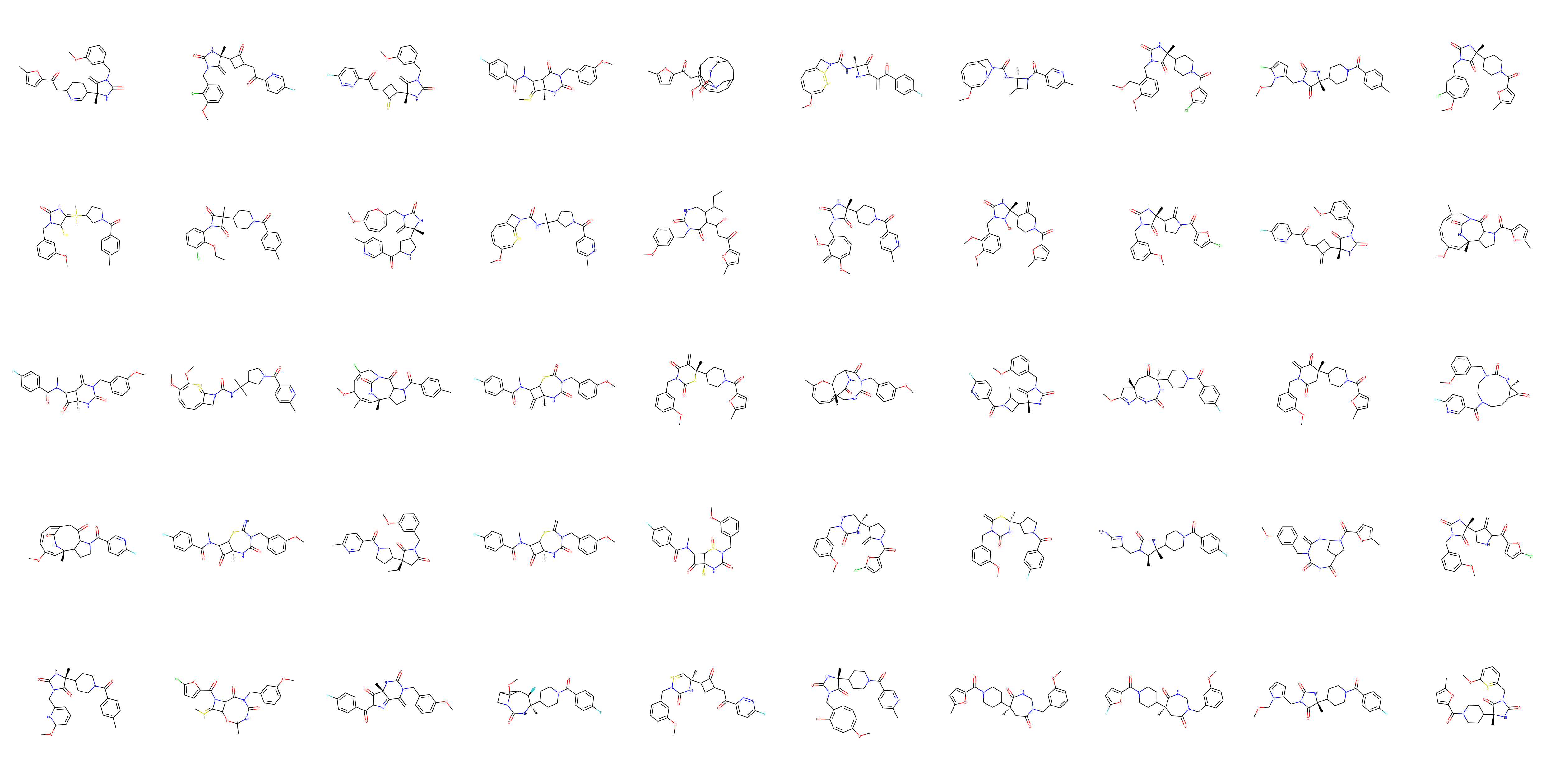
For this demonstration, I carried out the sampling procedure over 3 total rounds, starting from the best scoring structure from the initial optimization, to give 1166 unique structures. You will notice that the VAE decoded to some nonsense (not chemically reasonable) structures. However, it is a simple matter to filter such structures after the optimization.
# Generate local search space
smiles = mutate_search_space('COc1cccc(CN2C(=O)N[C@](C)(C3CCN(C(=O)c4ccc(C)nc4)CC3)C2=O)c1OC',
                             noise_norm=20.0,
                             decode_attempts=500,
                             n_mutations=2)

# Clean and normalize encoded data
domain = Data(smiles_to_z(smiles))
domain.clean()
domain.standardize(scaler='minmax', target=None)
Sample of structures:
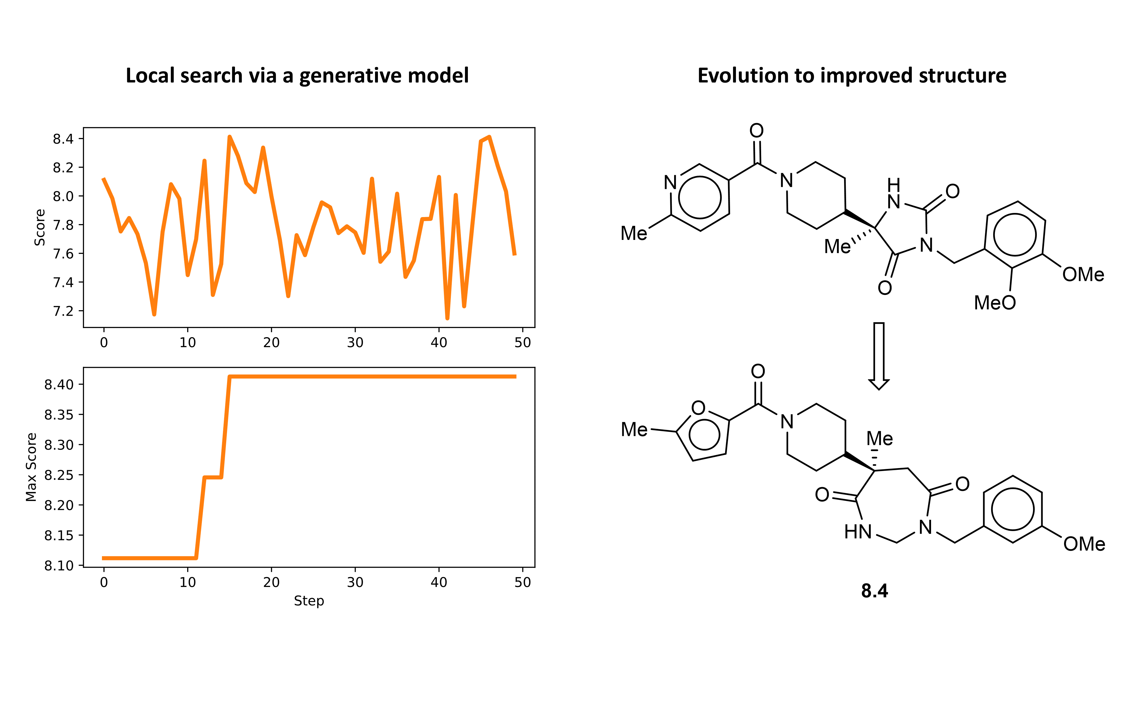
Finally, we can run the second round of optimization over this new domain using the same methodology as before. In this round the optimizer was able to discover several structures with predicted binding affinity at or above that of the best structure from the initial search. The structure with the highest predicted binding affinity and the optimization path is shown below.
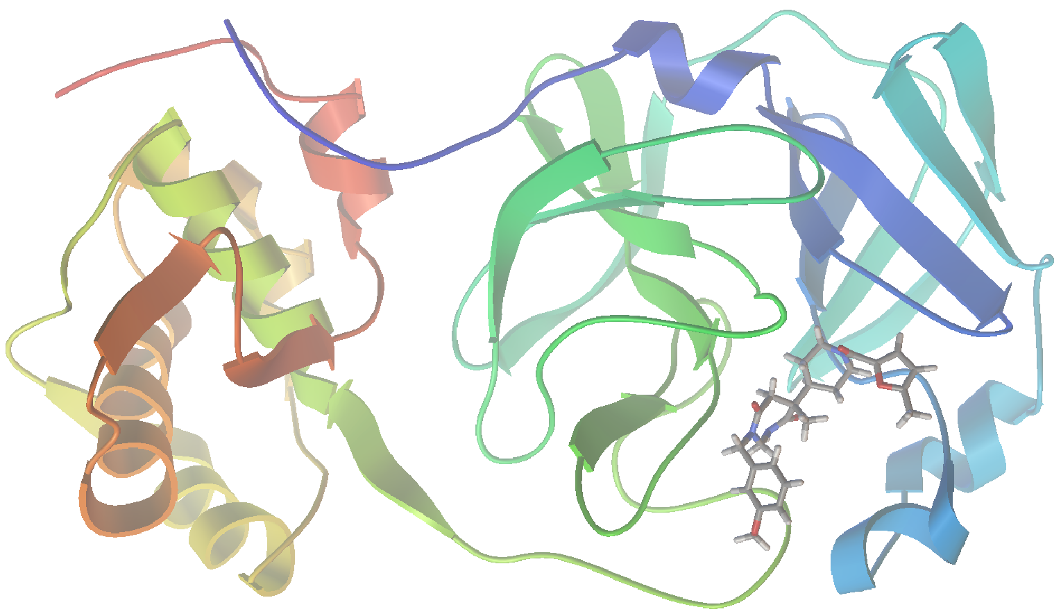
Once again, we can check out the results for the best ligand conformer using PMV.
This about wraps up our hands-on investigation of molecular docking. In this post, we have built a general and fully automated ligand discovery pipeline using molecular docking and ML. This system carries out molecular design (using a VAE), optimization (using BO), and scoring (via molecular docking and a RF model) using freely available and open-source software. As a demonstration, we utilized this approach to identify promising binders of the SARS-CoV-2 protease Mpro. Notably, the optimizer identified molecular structures with near nanomolar predicted binding affinity using a low-power laptop and evaluating < 100 candidate structures. Therefore, if this system were improved and scaled to include a larger search it is plausible that even more promising molecular structures could be identified. Finally, to put this demonstration in context, in a real drug development program it would next be up to synthetic chemists and biologists to experimentally validate such findings.
